Retip Logo

Retip - Retention Time Prediction for metabolomics

Paolo Bonini², Tobias Kind¹, Hiroshi Tsugawa³, Dinesh Barupal¹, Oliver Fiehn¹

Published 10 May 2020 in Analytical Chemistry

Please cite:

Retip: Retention Time Prediction for Compound Annotation in Untargeted Metabolomics Paolo Bonini, Tobias Kind, Hiroshi Tsugawa, Dinesh Kumar Barupal, and Oliver Fiehn Analytical Chemistry 2020 92 (11), 7515-7522 DOI: 10.1021/acs.analchem.9b05765

Retip 2.0 was updated and released in June 2024 by oloBion.

Introduction

Retip is a tool for predicting Retention Time (RT) for small molecules in a high pressure liquid chromatography (HPLC) Mass Spectrometry analysis, available as both an R package and a Python package. Retention time calculation can be useful in identifying unknowns and removing false positive annotations. The R package uses six different machine learning algorithms to built a stable, accurate and fast RT prediction model:

Random Forest: a decision tree algorithms.
BRNN: Bayesian Regularized Neural Network.
XGBoost: an extreme Gradient Boosting for tree algorithms.
lightGBM: a gradient boosting framework that uses tree based learning algorithms.
Keras: a high-level neural networks API for Tensorflow.
H2O autoML: an automatic machine learning tool.

Retip also includes useful biochemical databases like: HMDB, KNApSAcK, ChEBI, DrugBank, SMPDB, YMDB, T3DB, FooDB, NANPDB, STOFF, BMDB, LipidMAPS, Urine, Saliva, Feces, ECMDB, CSF, Serum, PubChem.1, PlantCyc, UNPD, BLEXP, NPA and COCONUT.

Get started

To use Retip, you need to prepare a compound retention time library in the format below. The input file needs compound Name, InChIKey, SMILES code and experimental retention time information for each compound. The input must be an MS Excel file. Retip will use this input file to build a the model and will predict retention times for other biochemical databases or an input query list of compounds. It is suggested that the file has at least 300 compounds to build a good retention time prediction model.

Input file view:

NAME	InChIKey	SMILES	RT
(2-oxo-2,3-dihydro-1H-indol-3-yl)acetic acid	ILGMGHZPXRDCCS-UHFFFAOYSA-N	C1=CC=C2C(=C1)C(C(=O)N2)CC(=O)O	2.019083
1,1-Dimethyl-4-phenylpiperazinium	WVHNHHJEHFWYHH-UHFFFAOYSA-N	CC1C(NC(CN1)C2=CC=CC=C2)C	2.60795
1,2-Cyclohexanediol	PFURGBBHAOXLIO-OLQVQODUSA-N	C1CCC@@HO	4.87655
1,2-Cyclohexanedione	OILAIQUEIWYQPH-UHFFFAOYSA-N	C1CCC(=O)C(=O)C1	5.772267
1,3,7-Trimethyluric acid	BYXCFUMGEBZDDI-UHFFFAOYSA-N	CN1C2=C(NC1=O)N(C(=O)N(C2=O)C)C	1.827733
1,3 Cyclohexanedione	HJSLFCCWAKVHIW-UHFFFAOYSA-N	C1CC(=O)CC(=O)C1	1.473133
1,4-Cyclohexanedicarboxylic acid	PXGZQGDTEZPERC-UHFFFAOYSA-N	C1CC(CCC1C(=O)O)C(=O)O	1.560217

In case, you want to avoid building a library from scratch, you can utilize publicly available libraries from Riken, Japan PlaSMA and the West Coast Metabolomics Center UC Davis, USA MoNA. Experimentation details for these two libraries are available here (link). We have already calculated retention time for several databases for these two experimental conditions.

If you would like that your retention time library to be included in Retip, please contact the Retip team (pb@olobion.ai).

Retip installation

Retip 2.0 requires R 4.4.0 and it is recommended to use RStudio IDE to run it.

Download and install R from the CRAN (64 bit version recommended)
Download and install RStudio
Download and install Java JDK

Run the following command lines to install Java in Ubuntu.

sudo apt update
sudo apt install default-jre
sudo apt install default-jdk
sudo R CMD javareconf

It is also possible that r-cran-rjava needs to be installed.

Download and install Rtools (Windows)
Download and install python3 (required to use Keras model)

Run the following command line to install python with R.

reticulate::install_python(version = 3.10)

Run the following command block to install all required packages, as well as the Retip packages and Retip library.

install.packages('rJava', repos='http://cran.rstudio.com/')

install.packages('devtools', version='2.4.5', repos='http://cran.rstudio.com/')
install.packages('caret', version='6.0-94', repos='http://cran.rstudio.com/')
install.packages('ggplot2', version='3.5.1', repos='http://cran.rstudio.com/')
install.packages('rcdk', version='3.8.1', repos='http://cran.rstudio.com/')
install.packages('rcdklibs', version='2.9', repos='http://cran.rstudio.com/')
install.packages('doParallel', version='1.0.17', repos='http://cran.rstudio.com/')
install.packages('stringi', version='1.8.4', repos='http://cran.rstudio.com/')
install.packages('lattice', version='0.22-5', repos='http://cran.rstudio.com/')
install.packages('randomForest', version='4.7-1.1', repos='http://cran.rstudio.com/')
install.packages('xgboost', version='1.7.7.1', repos='http://cran.rstudio.com/')
install.packages('brnn', version='0.9.3', repos='http://cran.rstudio.com/')
install.packages('lightgbm', version='4.3.0', repos='http://cran.rstudio.com/')
install.packages('h2o', version='3.44.0.3')
install.packages('gtable', version='0.3.5', repos='http://cran.rstudio.com/')
install.packages('grid', version='4.4.0', repos='http://cran.rstudio.com/')
install.packages('gridExtra', version='2.3', repos='http://cran.rstudio.com/')
install.packages('reticulate', version='1.37', repos='http://cran.rstudio.com/')

devtools::install_github('olobion/Retiplib')
devtools::install_github('olobion/Retip')

It is not possible to install Retip in conda enviroment because rJava requires NVIDIA drivers.

To make the package work fully in R, you need to install LightGBM, which can be very difficult. If you encounter problems, follow these instructions: LightGBM. If you do not need to use it, do not worry - you can continue using XGBoost, RandomForest, BRNN and H2O.

Retip workflow functions

To run the Retip workflow for an input compound library, following functions need to be called in a sequence.

prep.wizard
getCD
proc.data
chem.space
split training and testing
fit.model
get.score
p.model
p.model.features
RT.spell

Packages import

Set keras_installed = TRUE if you have installed keras.

setwd(setwd(dirname(rstudioapi::getActiveDocumentContext()$path)))
library(Retip)
keras_installed <- FALSE
if (!keras_installed) {
  keras::install_keras()
}

Set up Retip

First of all you have execute function prepare.wizard that is needed to activate the parallel computing to speed up models functions.

Then you have to import your custom excel file or use FiehnLab Hilic or Riken Plasma included library.

#>Starts parallel computing
prep.wizard()

# import excel file for training and testing data
rp2 <- readxl::read_excel("Plasma_positive.xlsx", sheet = "lib_2",
                          col_types = c("text", "text", "text", "numeric"))

#> or use HILIC database included in Retip
#> HILIC <- HILIC

Compute Chemical Descriptors with CDK

Now it is time to compute chemical descriptors with CDK a JAVA based open source project aimed at cheminformatics. Several core people around the Steinbeck group developed the code. According to Ohloh the development took 136 Person, several years and translated into several million dollars in development cost. For you will be simple as type getCD. Depending on your library length and your PC it will take few minutes to several hours. There is a counter to visualize the progress. It’s possible that the return table have less compounds respect the one you have start with. This is because some of yours smile code is not well formatted or for some compounds CDK is not able to calculate chemical descriptors. It is a pity but in real life happens that you have to leave behind even your favorite compound. If happens with most of compounds check SMILES, or better use Pubchem interchange service to get good working SMILES for your library.

Remember: clean your SMILES from salts and metal containing compounds before starting Retip to avoid cavities. You can use for this purpose ChemAxon standardizer, for example.

descs <- getCD(rp2)

Clean dataset

Some machine learning model did not like NA value, or low variance columns. So they are eliminated to improve model performance. This is done in Retip function proc.data.

#> Clean dataset from NA and low variance value
db_rt <- proc.data(descs)

Plot ChemSpace

You have now created your library with chemical descriptors. It is time to visualize your data and answer a two crucial question:

What do you want to predict?
Can I use my library to predict the whole Human Metabolome Database? Or PlantCyc?

The answer is not easy and pass trough another question: is the chemical space of my library large enough? So we have created function chem.space to plot your indulged data into chemical reality. You can chose a target between several database (HMDB, KNAPSACK, CHEBI, DRUGBANK, SMPDB, YMDB, T3DB, FOODB, NANPDB, STOFF, BMDB, LIPIDMAPS, URINE, SALIVA, FECES, ECMDB, CSF, SERUM, PUBCHEM.1, PLANTCYC, UNPD, BLEXP, NPA and COCONUT). In red you will see your library, in gray the chosen database.

Chemspace

Center and scale Optional - Warning

Centering and scaling can be useful for Keras model, but can decrease performance of others models. Actually is a very delicate step that you have to pay a lot of attention. Set cesc=TRUE if you want to perform this step. In that case, cesc input will be included when you predict your target database. It is necessary to avoid obtaining a completely wrong prediction.

Pay attention!

#> Optional center and scale data
#> this option improves Keras model
cesc <- FALSE
if (cesc) {
  # Build a model to use for center and scale a dataframe
  preproc <- cesc(db_rt)
  # use the above created model for center and scale dataframe
  db_rt <- predict(preproc, db_rt)
}

#> IMPORTANT : if you use this option remember to set cesc variable into
#> rt.spell and getRT.smile functions

Training and Testing set-up

A very important step is to split in training and testing your data frame.

Guide lines to build effective model explicitly specify: “QSAR/QSPR model have to be properly validated using data which was not in the training set”.

This is not new, is known from the Ancient Rome “divide et impera” (divide and conquer).

We can use caret function createDataPartition as follow:

#> Split in training and testing using caret::createDataPartition
set.seed(101)
in_training <- caret::createDataPartition(db_rt$XLogP, p = .8, list = FALSE)
training <- db_rt[in_training, ]
testing <- db_rt[-in_training, ]

Building QSAR models:

Now is time to put your hands on Retip ALMA mater: Advanced Learning Machine Algorithms.

Our suggestion is to compute all of them. Each function have an integrated tuning function to find out best parameters on your own library. Do not worry too much about over fitting because we have done 10 times fold cross validation. Each model have his advantage or disadvantage, it is simply depends on your data the one that fit better. Your models will be saved after building them so you can directly load them the next time that you open your project. Set buildModels=FALSE to load your previously built models.

Have fun!

build_models <- TRUE

if (build_models) {
  rf  <- fit.rf(training)
  saveRDS(rf, "rf_model.rds")

  brnn <- fit.brnn(training)
  saveRDS(brnn, "brnn_model.rds")

  keras <- fit.keras(training, testing)
  save_model_hdf5(keras, filepath = "keras_model.h5")

  lightgbm <- fit.lightgbm(training, testing)
  saveRDS(lightgbm, "lightgbm_model.rds")

  xgb <- fit.xgboost(training)
  saveRDS(xgb, "xgb_model.rds")
  
  aml <- fit.automl.h2o(training)
  # It saves by default the best model
  h2o::h2o.saveModel(aml@leader, "automl_h2o_model")
} else {
  xgb <- readRDS("xgb_model.rds")
  rf <- readRDS("rf_model.rds")
  brnn <- readRDS("brnn_model.rds")
  keras <- keras::load_model_hdf5("keras_model.h5")
  lightgbm <- readRDS("lightgbm_model.rds")
  h2o::h2o.init(nthreads = -1, strict_version_check=FALSE)
  aml <- h2o.loadModel("automl_h2o_model/###") # replace ### with the name of your saved model
}

Testing and plot models

Congratulations you have built your model!

Let’s see how much accurate it is. First of all check the scores with function get.score. Returns:

RMSE: root-mean-square error (the most important one)
R2: coefficient of determination
MAE: Mean Absolute Error
95% ± min: is the 95% confidence in minutes

The best model is always the first based on lower RMSE value. You can check only one model or all of them (maximum 6) at same time.

#> first you have to put the testing dataframe and then the name of the models
#> you have computed
stat <- get.score(testing, xgb, rf, brnn, keras, lightgbm, aml)
stat

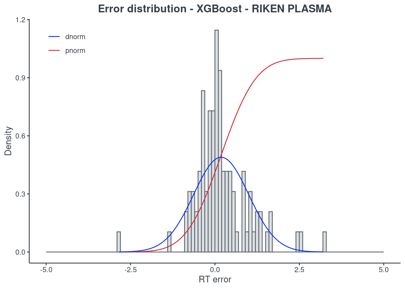
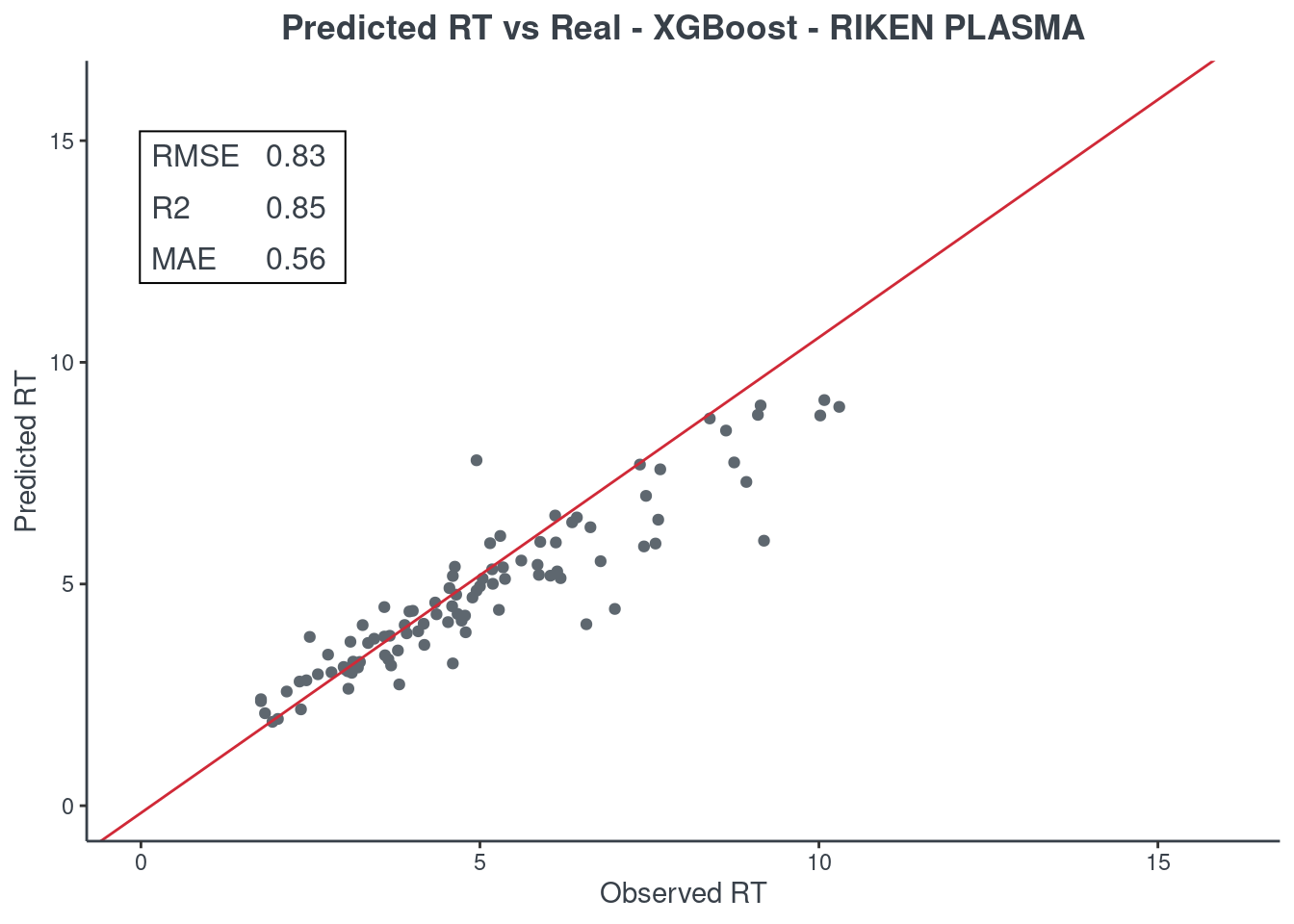
You can also visualize model performance using function p.model using testing dataframe as input. You can also use training data or whole data to see how it change, even if the only really important is the testing one.

XGBoost

#> first you have to put the testing daframe and then the name of the models
#> you want to visualize.
#> Last value is the title of the graphics.
p.model(testing, m = xgb, title = "XGBoost - RIKEN PLASMA")

error_xgboost predreal_xgboost

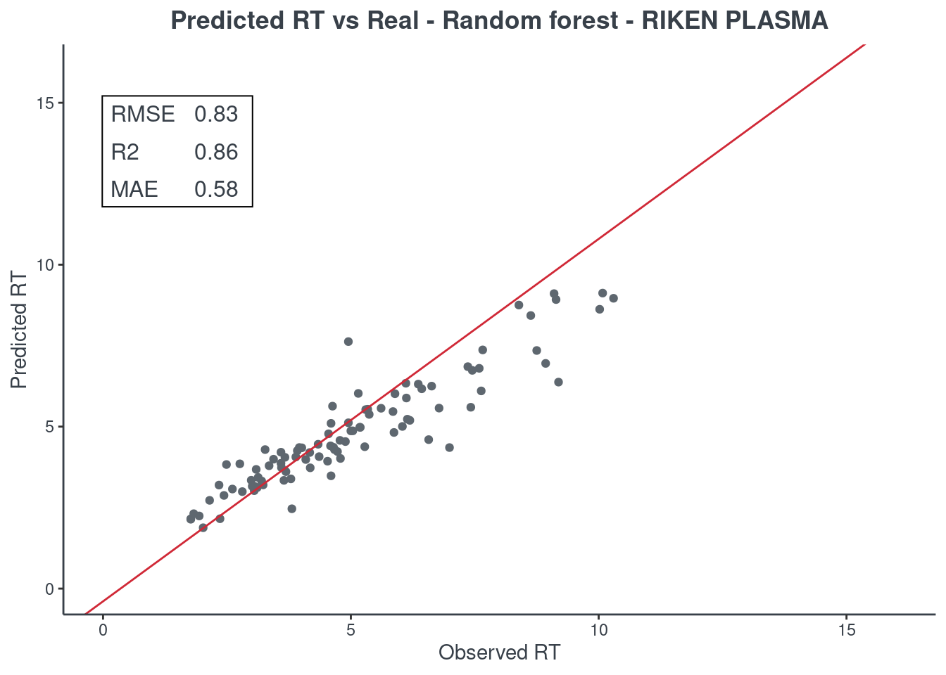
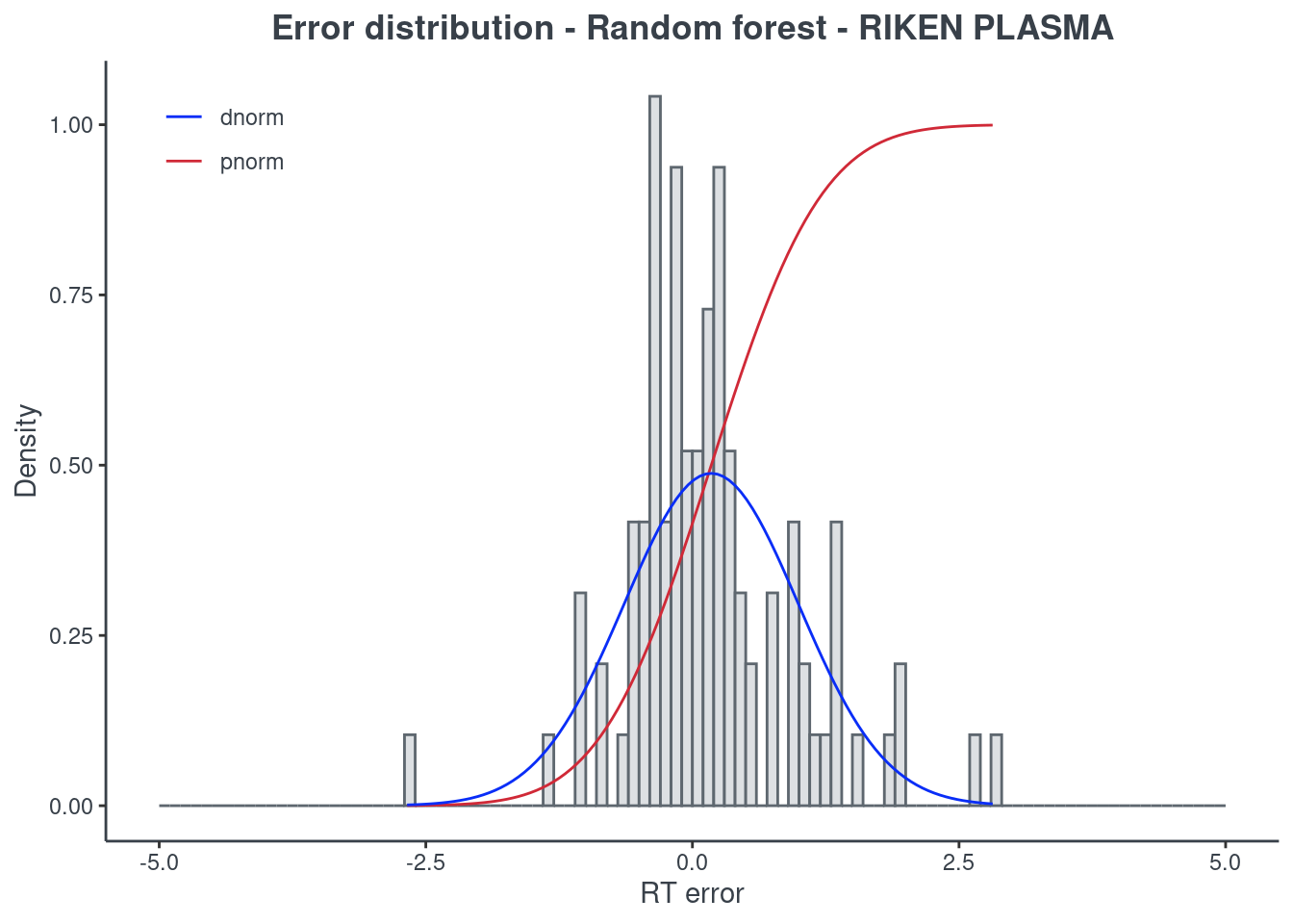
Random forest

#> first you have to put the testing daframe and then the name of the models
#> you want to visualize.
#> Last value is the title of the graphics.
p.model(testing, m = rf, title = "Random forest - RIKEN PLASMA")

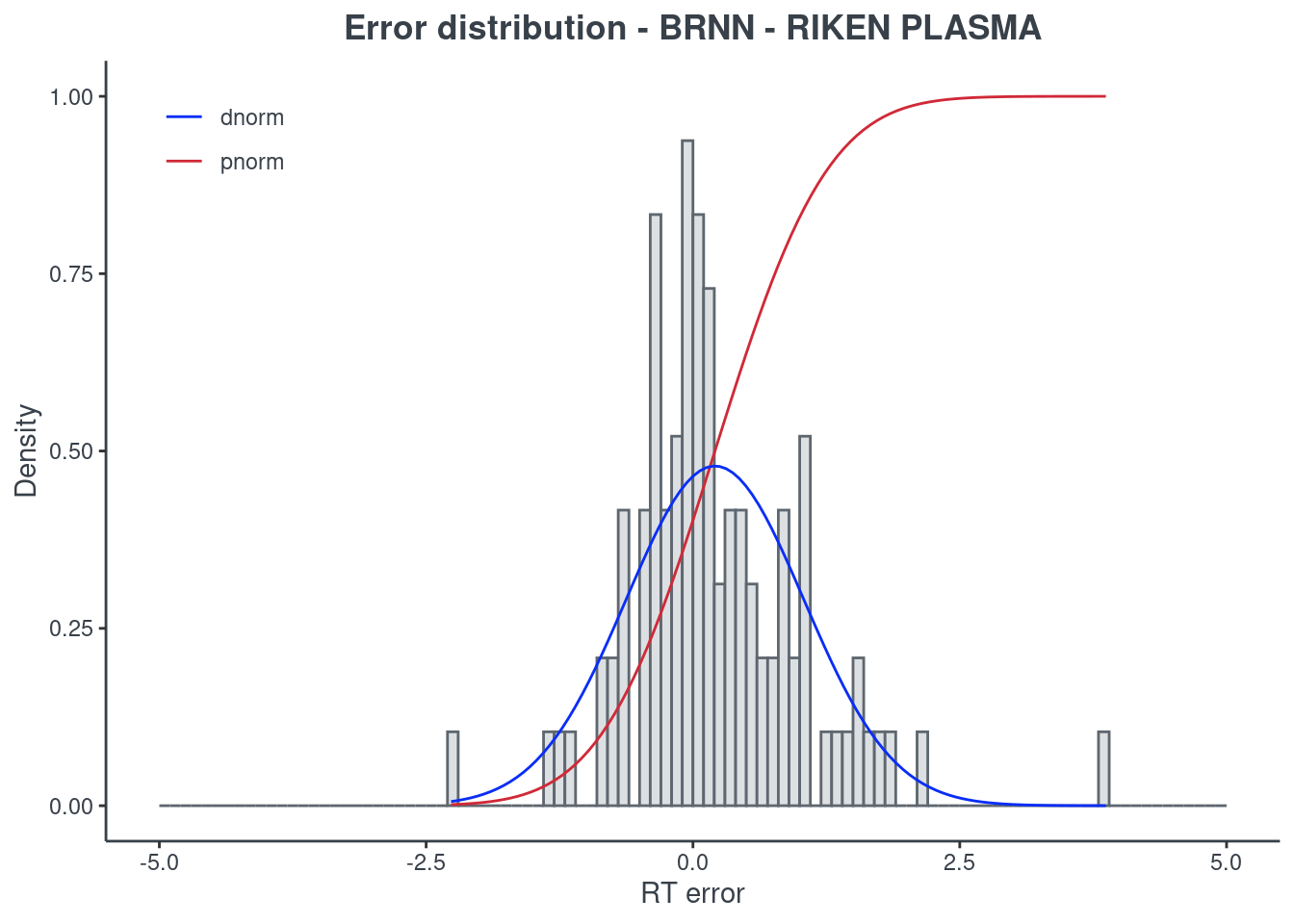
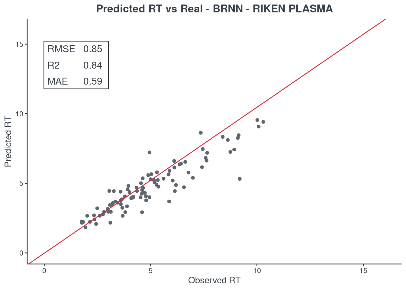
error_randomforest predreal_randomforest

BRNN

#> first you have to put the testing daframe and then the name of the models
#> you want to visualize.
#> Last value is the title of the graphics.
p.model(testing, m = brnn, title = "BRNN - RIKEN PLASMA")

error_brnn predreal_brnn

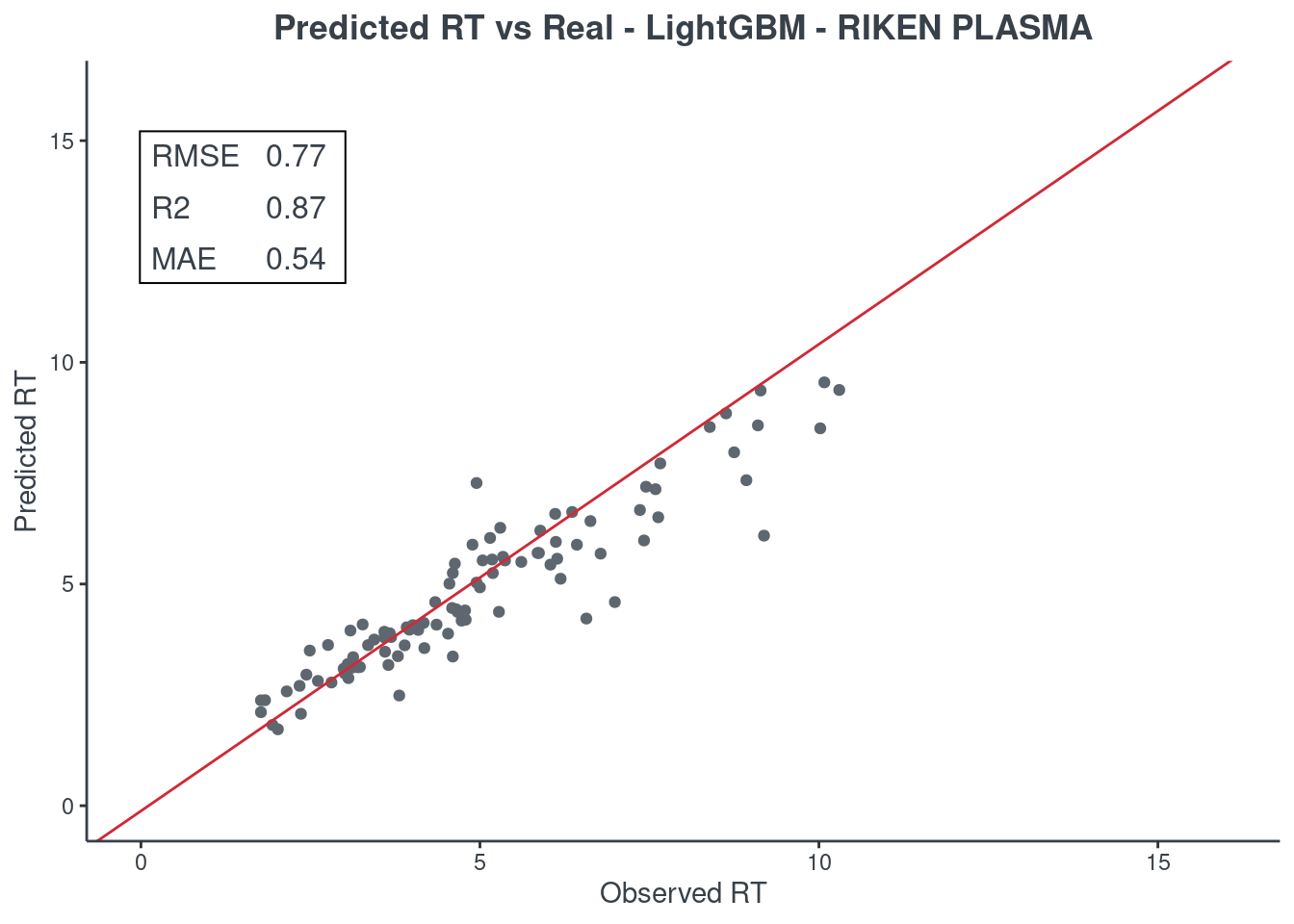
LightGBM

#> first you have to put the testing daframe and then the name of the models
#> you want to visualize.
#> Last value is the title of the graphics.
p.model(testing, m = lightgbm, title = "LightGBM - RIKEN PLASMA")

error_lightgbm predreal_lightgbm

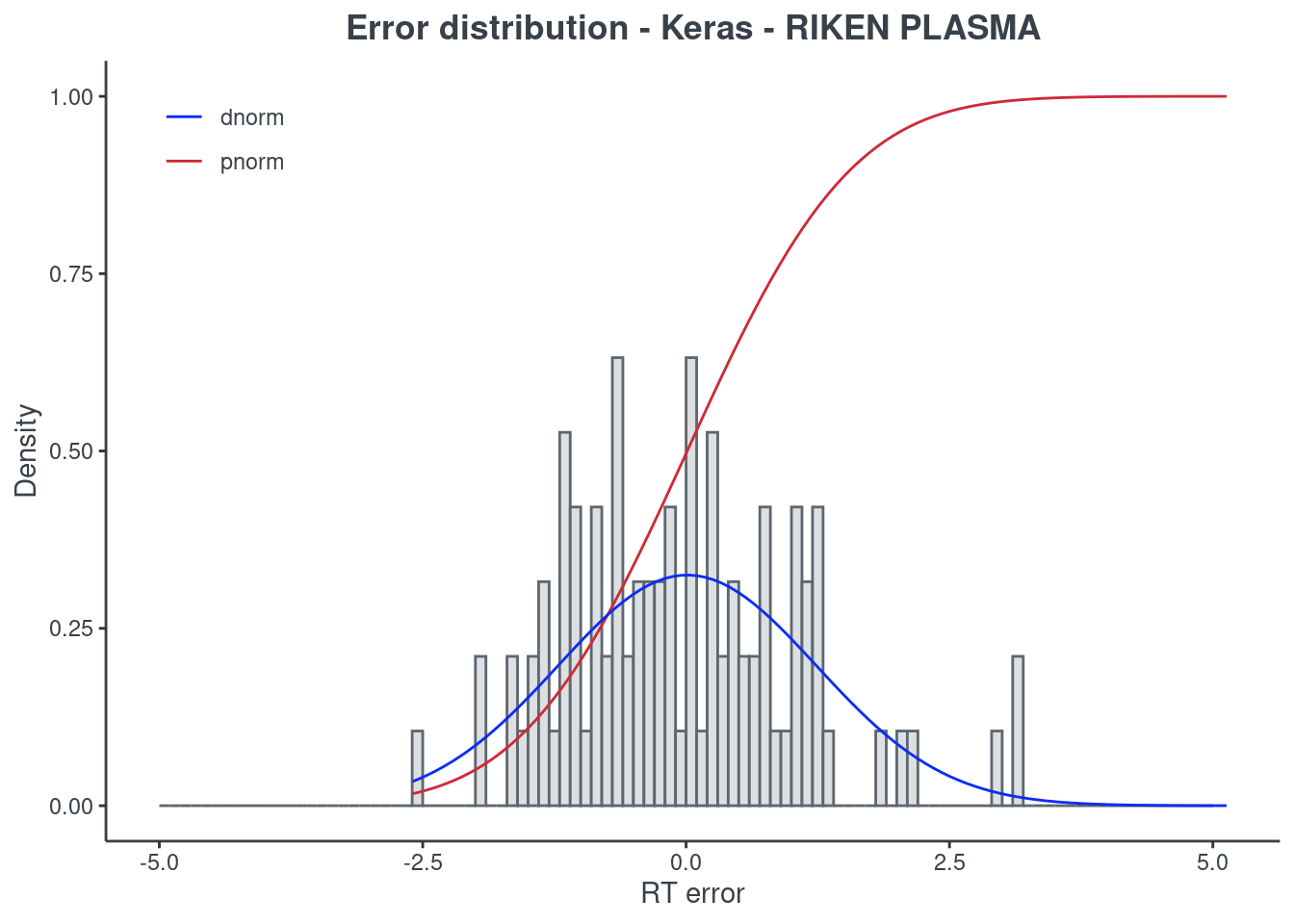
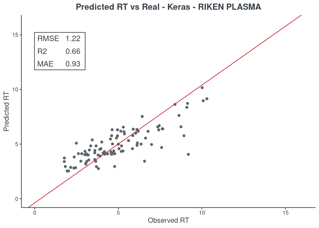
Keras

#> first you have to put the testing daframe and then the name of the models
#> you want to visualize.
#> Last value is the title of the graphics.
p.model(testing, m = keras, title = "Keras - RIKEN PLASMA")

error_keras predreal_keras

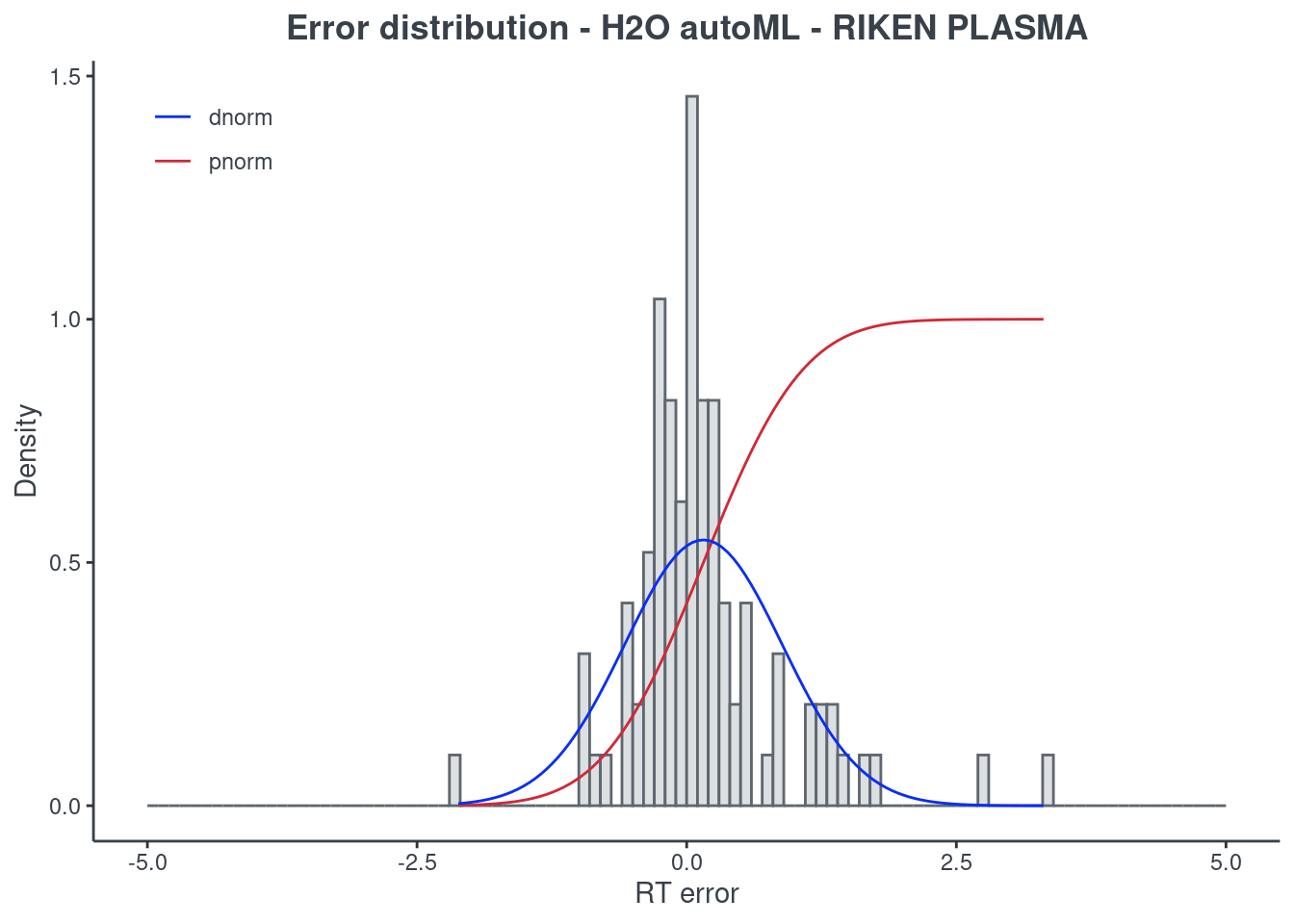
H2O autoML

#> first you have to put the testing daframe and then the name of the models
#> you want to visualize.
#> Last value is the title of the graphics.
p.model(testing, m = aml, title = "H2O autoML - RIKEN PLASMA")

error_h2o predreal_h2o

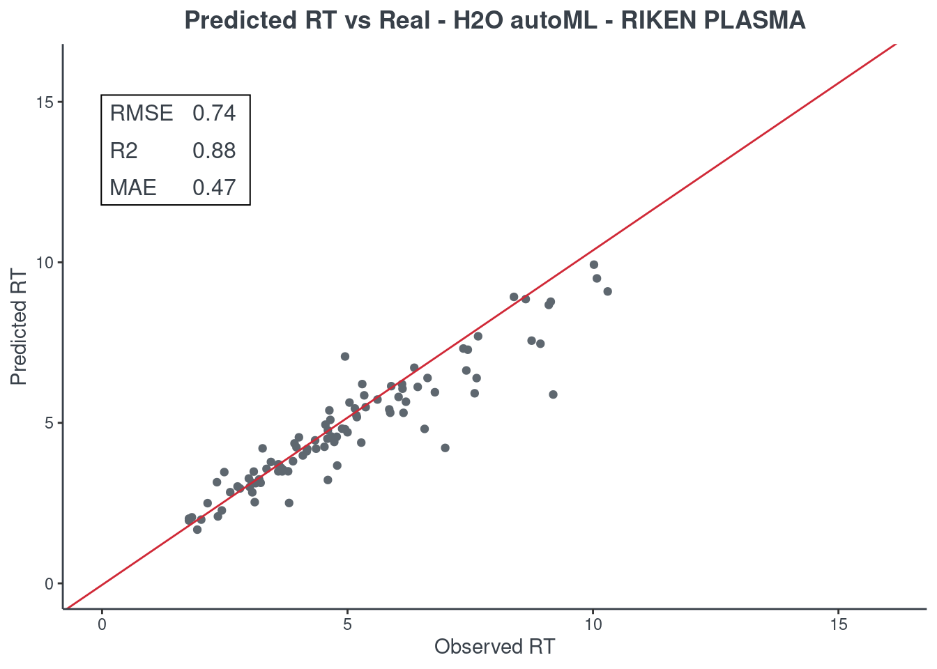
For the H2O autoML model, the statistics and the figures are obtained from the best model (aml@leader). If you want to check one of the other models, you have to select it using the model ID. The same applies when saving your H2O AutoML model. You will find an example of how to get a different model in the following command block.

#> First, get the leaderboard of your model
# aml_lb <- as.data.frame(h2o::h2o.get_leaderboard(object = aml, extra_columns = "ALL"))
#> Second, decide the model you want to inspect and select
#> The number corresponds to the index
# model_id <- aml_lb[3, "model_id"]
# selected_model <- h2o::h2o.getModel(model_id)

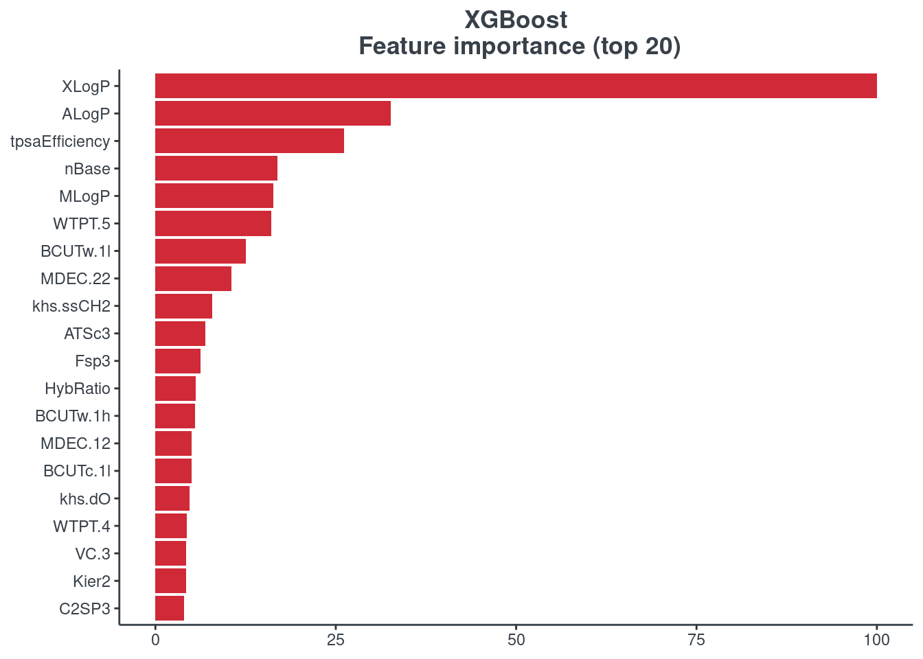
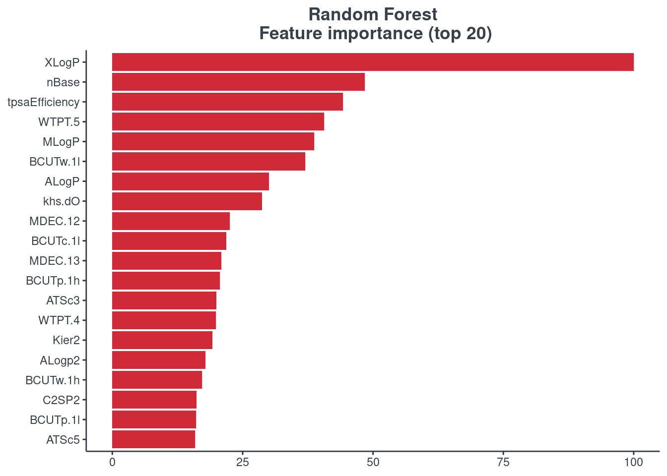
Feature importance

You can visualize the feature importance of your model using the p.model.features function. You have to indicate your model (model) and your model type (mdl_type). The accepted inputs for mdl_type are XGBoost (xgb), Random Forest (rf), BRNN (brnn), LightGBM (lightgbm) and H2O autoML (h2o). The Keras model is not supported.

XGBoost

p.model.features(xgb, mdl_type = "xgb")

features_xgboost

Random forest

p.model.features(rf, mdl_type = "rf")

features_randomforest

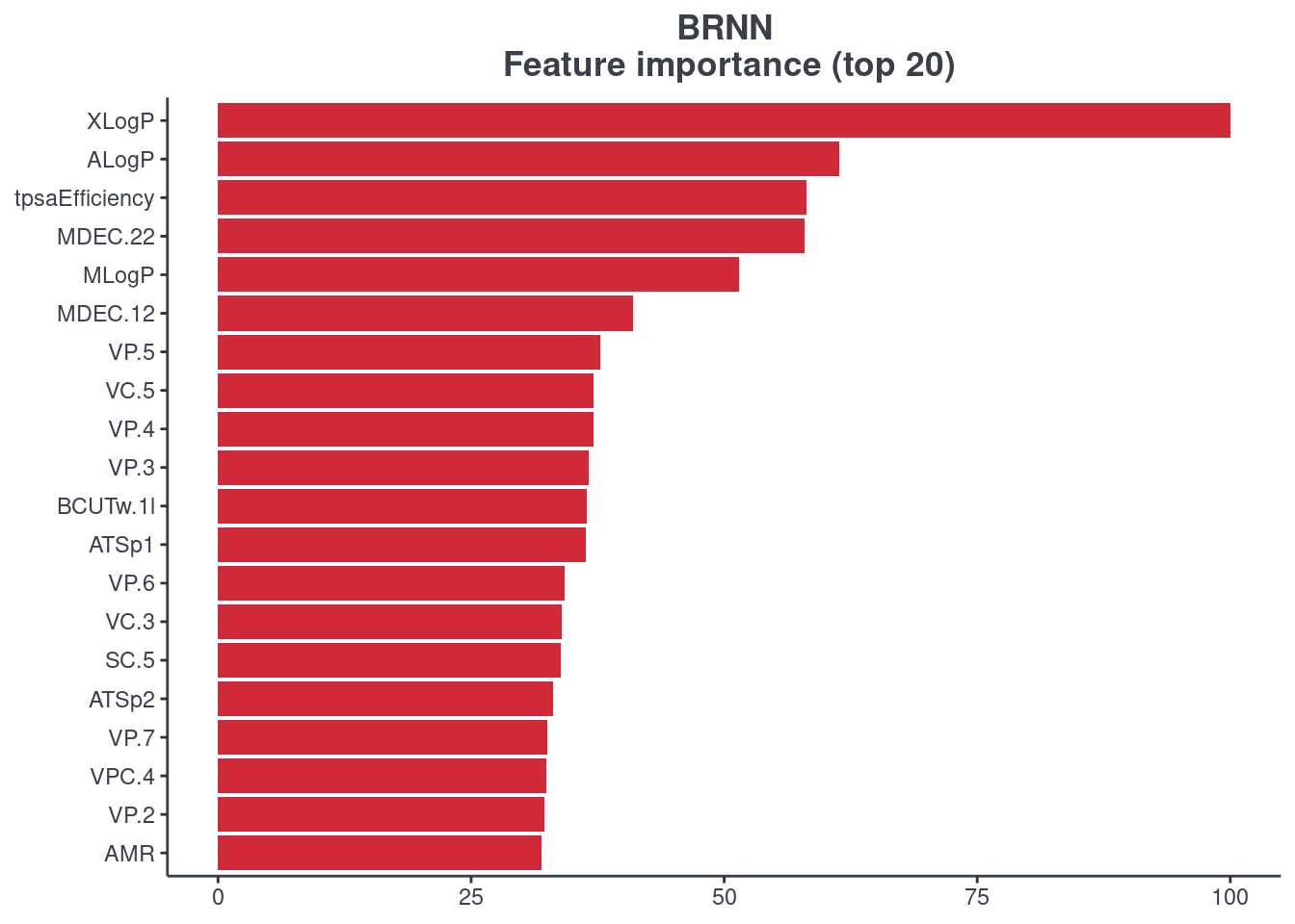
BRNN

p.model.features(brnn, mdl_type = "brnn")

features_brnn

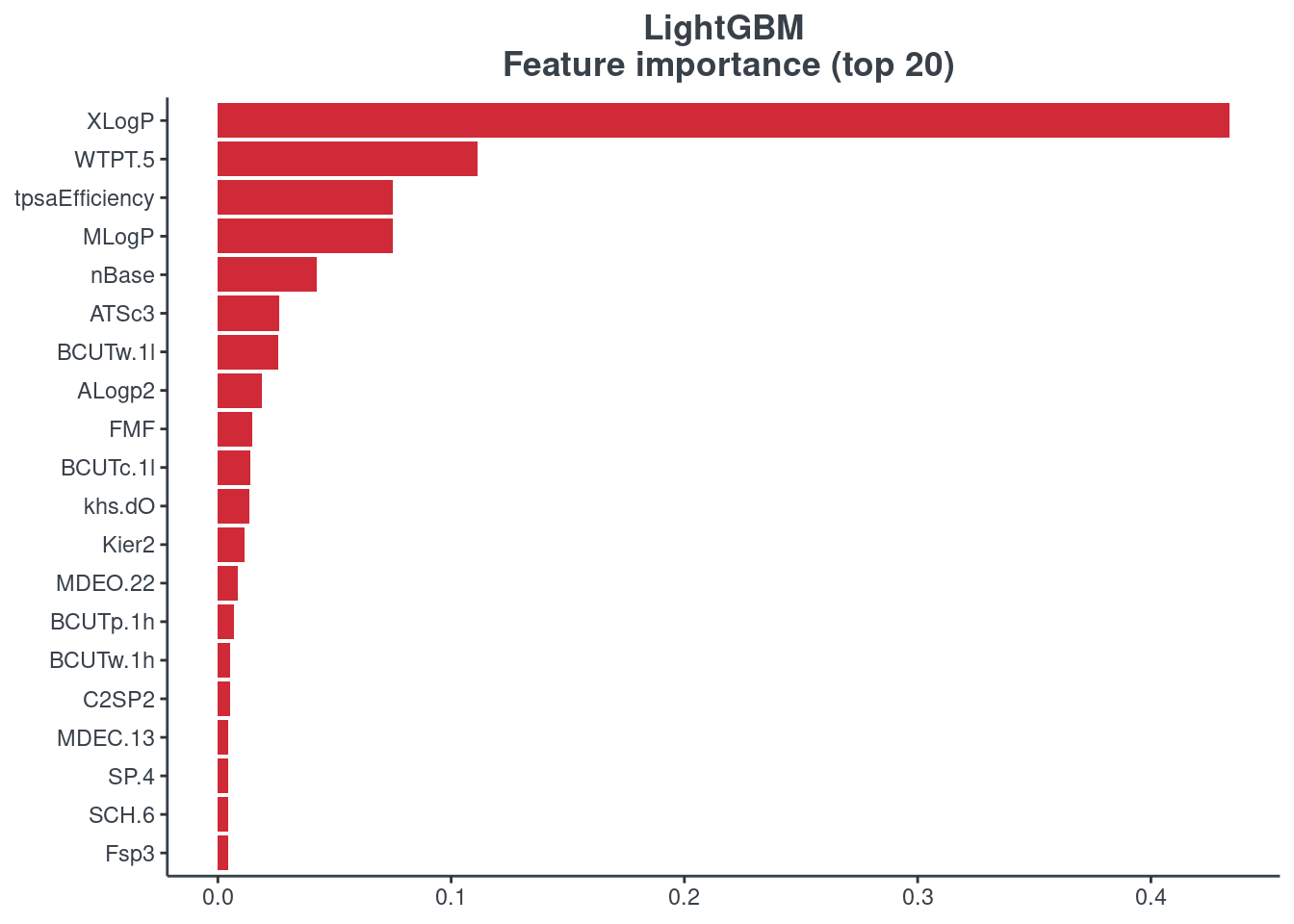
LightGBM

p.model.features(lightgbm, mdl_type = "lightgbm")

features_lightgbm

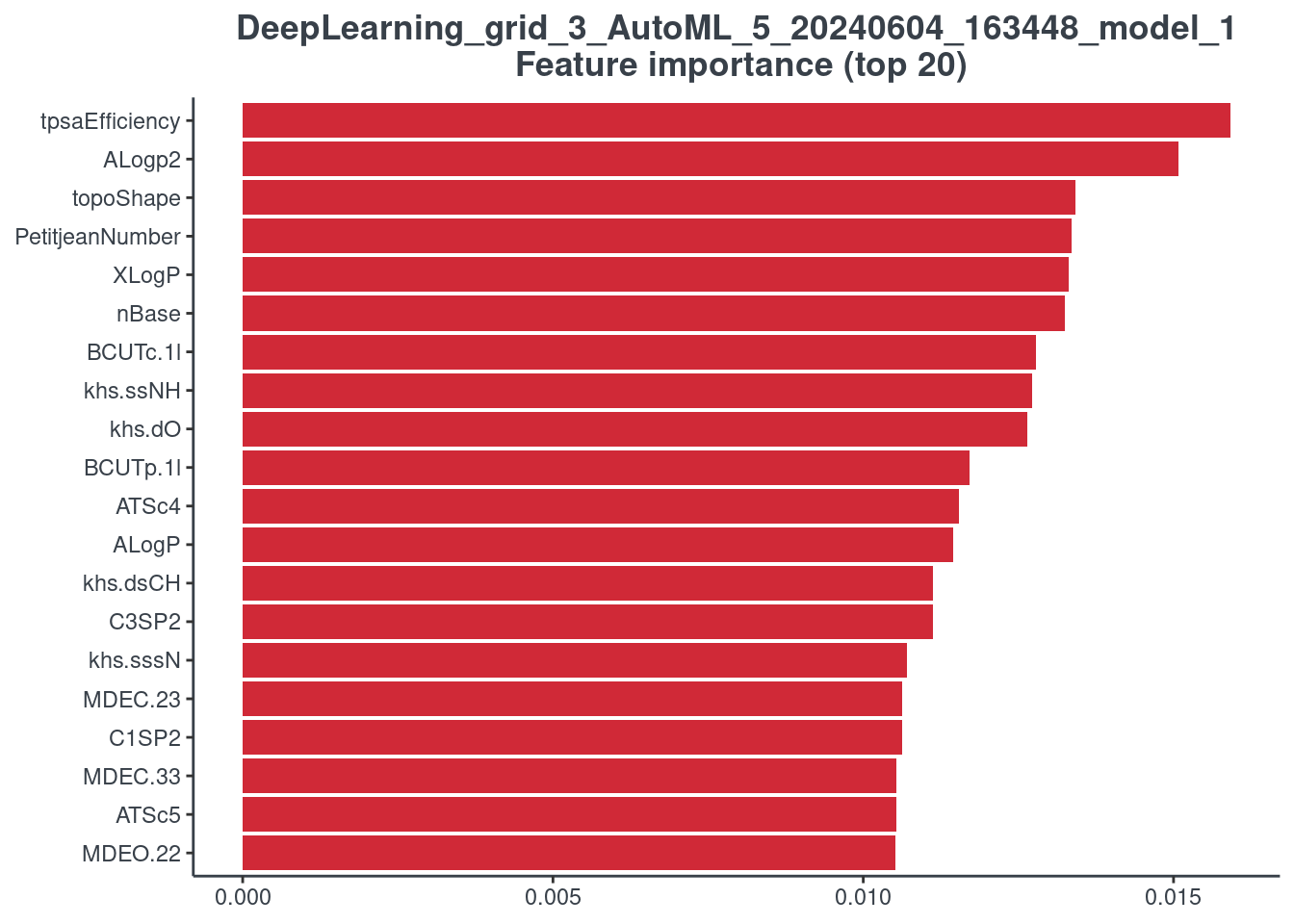
H2O autoML

It is not possible to plot the stacked ensemble models, but it is possible to plot the best 20 models used to construct the stacked one. For this reason, you have to indicate the number of the model (h2o_number) you want to see. You can find the correspondence between model ID and number running the following command line.

# aml_model_number <- as.data.frame(rownames(h2o::h2o.varimp(aml)))

p.model.features(aml, mdl_type = "h2o", h2o_number = 1)

features_h2o

Retention Time Prediction SPELL

This is the the final step. All the effort made before have been accomplished to compute the prediction on a whole database.

You have 3 options to make a prediction:

for your personal database
for downloaded mona.msp
for a Retip included database

1. Personal database

In that case, you have to import your excel with compound Name, InChIKey and SMILES code, compute CD and then make the prediction.

# import excel file for external validation set
rp_ext <- readxl::read_excel("Plasma_positive.xlsx", sheet = "ext",
                             col_types = c("text", "text", "text", "numeric"))
#> compute Chemical descriptors
rp_ext_desc <- getCD(rp_ext)

Clean data set from NA and low variance values using the Retip function proc.data as you did before with your data.

#> Clean dataset from NA and low variance value
db_rt_ext <- proc.data(rp_ext_desc)

Center and scale your data if you performed this step before.

if (cesc) {
  # Build a model to use for center and scale a dataframe
  preproc_ext <- cesc(db_rt_ext)
  # use the above created model for center and scale dataframe
  db_rt_ext <- predict(preproc_ext, db_rt_ext)
}

XGBoost

#> perform the RT spell
if (cesc) {
  rp_ext_pred_xgb <- Retip::RT.spell(training, rp_ext_desc, model = xgb,
                                     cesc = preproc)
} else {
  rp_ext_pred_xgb <- Retip::RT.spell(training, rp_ext_desc, model = xgb)
}

Random forest

#> perform the RT spell
if (cesc) {
  rp_ext_pred_rf <- Retip::RT.spell(training, rp_ext_desc, model = rf,
                                    cesc = preproc)
} else {
  rp_ext_pred_rf <- Retip::RT.spell(training, rp_ext_desc, model = rf)
}

BRNN

#> perform the RT spell
if (cesc) {
  rp_ext_pred_brnn <- Retip::RT.spell(training, rp_ext_desc, model = brnn,
                                      cesc = preproc)
} else {
  rp_ext_pred_brnn <- Retip::RT.spell(training, rp_ext_desc, model = brnn)
}

LightGBM

#> perform the RT spell
if (cesc) {
  rp_ext_pred_lightgbm <- RT.spell(training, rp_ext_desc, model = lightgbm,
                                   cesc = preproc)
} else {
  rp_ext_pred_lightgbm <- RT.spell(training, rp_ext_desc, model = lightgbm)
}

Keras

#> perform the RT spell
if (cesc) {
  rp_ext_pred_keras <- RT.spell(training, rp_ext_desc, model = keras,
                                cesc = preproc)
} else {
  rp_ext_pred_keras <- RT.spell(training, rp_ext_desc, model = keras)
}

H2O autoML

#> perform the RT spell
if (cesc) {
  rp_ext_pred_aml <- RT.spell(training, rp_ext_desc, model = aml,
                                cesc = preproc)
} else {
  rp_ext_pred_aml <- RT.spell(training, rp_ext_desc, model = aml)
}

2. Downloaded mona.msp

Here, you have to put your msp downloaded from Mona inside your project folder. First, prep.mona function is needed to extract information from msp file and build input table. Then, you have to compute CD using getCD, make the prediction and incorporate again inside msp file. In this way the msp file you have in your project folder is ready to be used for compound identification with MSMS and Retention time prediction.

db_mona <- prep.mona(msp = "MoNA-export-CASMI_2016.msp")

mona <- getCD(db_mona)

XGBoost

if (cesc) {
  mona_rt_xgb <- RT.spell(training, mona, model = xgb, cesc = preproc)
} else {
  mona_rt_xgb <- RT.spell(training, mona, model = xgb)
}

addRT.mona(msp = "MoNA-export-CASMI_2016.msp", mona_rt_xgb)

Random forest

if (cesc) {
  mona_rt_rf <- RT.spell(training, mona, model = rf, cesc = preproc)
} else {
  mona_rt_rf <- RT.spell(training, mona, model = rf)
}

addRT.mona(msp = "MoNA-export-CASMI_2016.msp", mona_rt_rf)

BRNN

if (cesc) {
  mona_rt_brnn <- RT.spell(training, mona, model = brnn,
                           cesc = preproc)
} else {
  mona_rt_brnn <- RT.spell(training, mona, model = brnn)
}

addRT.mona(msp = "MoNA-export-CASMI_2016.msp", mona_rt_brnn)

LightGBM

if (cesc) {
  mona_rt_lightgbm <- RT.spell(training, mona, model = lightgbm,
                               cesc = preproc)
} else {
  mona_rt_lightgbm <- RT.spell(training, mona, model = lightgbm)
}

addRT.mona(msp = "MoNA-export-CASMI_2016.msp", mona_rt_lightgbm)

Keras

if (cesc) {
  mona_rt_keras <- RT.spell(training, mona, model = keras,
                            cesc = preproc)
} else {
  mona_rt_keras <- RT.spell(training, mona, model = keras)
}

addRT.mona(msp = "MoNA-export-CASMI_2016.msp", mona_rt_keras)

H2O autoML

if (cesc) {
  mona_rt_aml <- RT.spell(training, mona, model = aml,
                            cesc = preproc)
} else {
  mona_rt_aml <- RT.spell(training, mona, model = aml)
}

addRT.mona(msp = "MoNA-export-CASMI_2016.msp", mona_rt_aml)

3. Retip included database

This option is the easiest one. We computed more than 300k compounds to save your time and more important save electricity (we love nature). You have just to chose a target database, the type of output and the polarity (pos or neg).

The available outputs are:

MSDIAL: identification with accurate Mass and RTP (RECOMMENDED); get MSDIAL
MSFINDER: identification with accurate Mass, in silico fragmentation MS2 and RTP (RECOMMENDED); get MSFINDER
AGILENT: works with Mass Hunter software
THERMO
WATERS
SCIEX

XGBoost

#> example of all Retip included compounds predicted and exported to MSFINDER
if (cesc) {
  all_pred_xgb <- RT.spell(training, target = "ALL", model = xgb,
                           cesc = preproc)
} else {
  all_pred_xgb <- RT.spell(training, target = "ALL", model = xgb)
}

export_rtp <- RT.export(all_pred_xgb, program = "MSFINDER", pol = "pos")

Random forest

#> example of all Retip included compounds predicted and exported to MSFINDER
if (cesc) {
  all_pred_rf <- RT.spell(training, target = "ALL", model = rf,
                          cesc = preproc)
} else {
  all_pred_rf <- RT.spell(training, target = "ALL", model = rf)
}

export_rtp <- RT.export(all_pred_rf, program = "MSFINDER", pol = "pos")

BRNN

#> example of all Retip included compounds predicted and exported to MSFINDER
if (cesc) {
  all_pred_brnn <- RT.spell(training, target = "ALL", model = brnn,
                            cesc = preproc)
} else {
  all_pred_brnn <- RT.spell(training, target = "ALL", model = brnn)
}

export_rtp <- RT.export(all_pred_brnn, program = "MSFINDER", pol = "pos")

LightGBM

#> example of all Retip included compounds predicted and exported to MSFINDER
if (cesc) {
  all_pred_lightgbm <- RT.spell(training, target = "ALL", model = lightgbm,
                                cesc = preproc)
} else {
  all_pred_lightgbm <- RT.spell(training, target = "ALL", model = lightgbm)
}

export_rtp <- RT.export(all_pred_lightgbm, program = "MSFINDER", pol = "pos")

Keras

#> example of all Retip included compounds predicted and exported to MSFINDER
if (cesc) {
  all_pred_keras <- RT.spell(training, target = "ALL", model = keras,
                             cesc = preproc)
} else {
  all_pred_keras <- RT.spell(training, target = "ALL", model = keras)
}

export_rtp <- RT.export(all_pred_keras, program = "MSFINDER", pol = "pos")

H2O autoML

#> example of all Retip included compounds predicted and exported to MSFINDER
if (cesc) {
  all_pred_aml <- RT.spell(training, target = "ALL", model = aml,
                             cesc = preproc)
} else {
  all_pred_aml <- RT.spell(training, target = "ALL", model = aml)
}

export_rtp <- RT.export(all_pred_aml, program = "MSFINDER", pol = "pos")

Conclusions Remarks:

Remember these few tips:

Split your data into training and testing (80/20). If you want to be cool use also an additional external dataset.
Do not cheat yourself doing cherry picking with testing molecules that are out-liner and putting in training data. Leave at it is, is better know the truth than lie to yourself.
As you probably know R use set.seed when you have a random function. This is needed to get the same results when you do it again. There is a set seed before the split training/testing. If you modify you get a slightly different results in your models if the problematic compounds are inside training data. This is not a real cheat because is random driven ;-)
Look at your smiles before import in Retip, if you have cavities in it will not work properly.

Remember Leonardo Da Vinci suggestion:

I have been impressed with the urgency of doing. Knowing is not enough; we must apply. Being willing is not enough; we must do.

Retip born to helps you in identification in metabolomics workflow, it is not an exhibition of knowledge. The success of this app is if helps in your work, in real world metabolomics experiments.